

Up to this point in calculus, we’ve been studying limits. Now, we are going to shift gears to the next major topic of calculus: derivatives.
In this video, we will introduce derivatives by discussing their formal definition and formula, mastering the first type of derivative problem, and exploring some real-world applications of this knowledge.
Derivative Formula
Suppose we have a graph of a function such as this one, and suppose we are interested in finding the tangent line at a given point.
When I say tangent line, I’m talking about the straight line that touches only that exact point of the function. For example, at this point, the tangent line would look like this.
Or at this point, the tangent line would look like this.
Again, the tangent line can only touch the function at that one point. Additionally, notice that from these examples, the tangent line must have the same slope as the function does at that exact point. So this would not be an example of a tangent line because it has a different slope than the function, which would cause it to intersect with the function in a second spot.
So a tangent line gives an indication of the slope of a function at a specific point. How would we find that precise value, though, apart from drawing the line by hand or by making guesses?
That answer can be found by using the derivative formula, which is:
The letters “\(f’x\)” are typically pronounced “\(f\) prime of \(x\)” and they refer to the function that describes the slope of \(f\) at the point \(x\). \(f\)’ and this concept of finding the slope at a specific point are key to the topic of derivatives.
Examples
Example #1
Let’s apply the derivative formula to an example. Find the function \(f\)’ describing the slope of \(f(x)=3x\).
So to find our derivative, we can use our derivative formula. So let’s write that out so that we can remember it. Our derivative formula is:
So now we’re going to use our function, \(f(x)\), to plug in our values into our formula and solve. We’re going to plug in \(x+h\) anywhere we see an \(x\) in our function.
This may look complex, but we can simplify the numerator before we need to bother with the limit. Distributing the 3 over \((x+h)\), we get \(3x + 3h – 3x\) in the numerator. The \(3x\)’s cancel each other out, leaving \(3h\) over \(h\).
From here, the two \(h\)’s cancel out, leaving us with:
The limit of any constant is that constant, so our answer is 3. Intuitively, we already knew this to be true because m, the slope of the line, was set to equal 3.
\(f(x)=3x+0\)
\(m=3\)
So \(f'(x)\), or our derivative of the function \(3x\), is equal to 3.
Example #2
Let’s try applying the derivative formula to another function. Find the function \(f’\), which describes the slope of \(f(x)=x^{2}\).
We’re going to start by writing out our derivative formula.
So for \(f(x+h)\), we’re going to plug in \(x+h\) anywhere we see an \(x\) in our original function.
Before worrying about the limit, we are going to again simplify the numerator as far as we can. First, FOIL out \((x+h)^{2}\).
\(f'(x)=\)\(\displaystyle \lim_{h \to 0}\frac{x^{2}+2xh+h^{2}-x^{2}}{h}\)
So now we can simplify this just a little bit. Our \(x^{2}\)’s will cancel each other out because one is positive and one is negative, and \(xh\) and \(hx\) are actually the same term, so we can simplify this to:
Now, from both terms in the numerator we can factor out an \(h\).
This \(h\) cancels out with the one in the denominator, so we are left with:
We can’t simplify this any further before dealing with the limit. Fortunately for us, though, this one is pretty easy. As \(h\) gets smaller and smaller toward zero, we approach \(2x\). So
Let’s see how our solution holds up. The graph of \(f(x)=x^{2}\) looks like this.
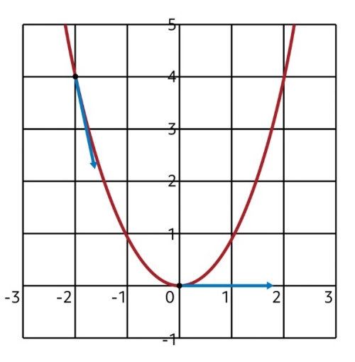
At the point \(x=0\), the slope should equal \(f'(0)=2(0)=0\). Sure enough, the curve is flat at that exact point!
Similarly, at the point \(x=-2\), the slope will be equal to \(f'(-2)=2(-2)=-4\). We can draw the tangent line and see that this is correct! Feel free to check the solution on your own at additional points.
Why the Formula Works
Now that we know how to apply the derivative formula, I want to briefly explain why it works. Let’s look at the formula again.
Remember when you learned about slope in algebra? The way we calculated a slope then was dividing the change in height by the change over the \(x\)-axis. Some students use the phrase “rise over run” to remember this relationship.
Here, the numerator of the derivative formula helps us calculate the change in height between the two points on the curve (the “rise”). Then, the denominator \(h\) describes how far along the \(x\)-axis we are moving (the “run”). So the fraction within the limit is itself a way of describing slope, because we can look at it as another way of saying “rise over run.”
Now, the limit tells us that h must get smaller and smaller toward zero. This means that we are considering the slope in smaller and smaller increments, and getting closer and closer to finding the instantaneous slope of the function.
Now that we have used the derivative formula a couple times, we can see that it typically isn’t difficult to use. Just plug everything in, simplify, and then take the limit.
The Power Rule
But there’s something I haven’t shared with you about derivatives yet: there’s an easier and faster way to solve for \(f'(x)\).
The trick I’m about to show you is called the power rule. It states that whenever a function \(f(x) \)is in the form \(x\) raised to some power \(n\), then \(f'(x)(x)\) is equal to \(n\) multiplied by \(x\) raised to one less power.
Going back to our first example in the video, we had the function \(f(x)=3x\) and computed its derivative using the derivative formula. Let’s solve for \(f’\) again now, using the Power Rule this time.
Even though \(f(x)\) has a coefficient of 3, we can still apply the Power Rule because it has \(x\) raised to some power \(n\). In this case, \(n=1\). So
\(f'(x)=3\cdot 1x^{1-1}\)
\(f'(x)=3x^{0}\)
\(f'(x)=3\)
This is exactly what we got earlier using the derivative formula!
Now, let’s apply the power rule to the other example from earlier: finding the derivative of \(f(x)=x^{2}\). In this case, \(x\) is raised to the second power, so \(n=2\). Plugging this into the formula, we have:
\(f'(x)=2x^{2-1}\)
\(f'(x)= 2x\)
This is the same solution we got earlier by using the derivative formula.
Real-World Example
I want to finish this lesson with a real-life example. One thing about derivatives that makes them fascinating is that they perfectly describe the relationship between speed and displacement, particularly when speed is varying. For example, if you are given a function that describes an object’s displacement, you can also determine the object’s speed by taking the derivative of the displacement function.
Let’s use this knowledge to work a real-life example. A soap box derby car’s displacement in feet is described by the following function, where x is in seconds: \(f(x)=\frac{1}{4}x^{2}+x\). Determine the car’s speed at 5 seconds by first using the Power Rule to find \(f'(x)\) and then evaluating at \(x=5\).
Our first step is finding \(f'(x)\) by using the Power Rule. Notice that \(f(x)\) has two terms, \(\frac{1}{4}x^{2}\) and \(x\). This is nothing to be concerned about; we will simply handle them one at a time. For the first term, \(x\) is raised to the second power, so \(n=2\). Then the derivative of this term will be
Now the second term is just \(x\), which is understood to be raised to the first power. By the Power Rule, we multiply this 1 in front of the \(x\), then reduce \(x\)’s power by 1.
So the reason that I just added the derivatives of these two functions was because of what’s called the sum rule for derivatives. So that says that if you have a sum of two different parts of a function, you can then take both of those parts’ derivatives and add them together, just like we did.
We now have the speed function:
All we have to do from here is plug in \(x=5\) to find the car’s speed at five seconds.
\(f'(x)=\frac{5}{2}+1\)
\(f'(5)=\frac{7}{2}=3.5\)
So at 5 seconds, the car is moving at 3.5 feet per second.
As we’ve seen in this video, derivatives can be calculated using the derivative formula or by applying the power rule, whenever the terms of \(f\) are in the form \(x\) raised to some power.
Now you have the tools you need to start working on derivatives yourself!
Thanks for watching, and happy studying!