

What are limits? How do we use them? And what do they tell us? In this video, we are going to take a broad look at limits, briefly touching on each of the more important matters related to this important unit of calculus.
The Problem of Undefined Functions
To get an idea of the usefulness of limits, let’s start by looking at an algebra problem.
Evaluate the function \(f(x)=\frac{3x^{2}-5x-2}{x-2}\) at \(x=2\).
At first glance, no problem, right? Look again. What happens when we plug in \(x=2\) into the denominator? We get 0. And this is a problem!
As I’m sure you’re aware, dividing anything by 0 is undefined in mathematics, so \(f(2)\) does not exist at all!
Limit Notation
That’s where limits come in. Limits help us observe the behavior of functions around “trouble spots” like. In this case, \(x=2\). Continuing with the same function \(f(x)\), let’s see exactly how limits can work.
Before we dive in though, it’s important for us to establish notation. Limit notation looks like this:
“lim” is an abbreviation for “limit”, and below it, we write our independent variable \(x\), an arrow, and the value of \(x\) we are particularly concerned with. To the right of this, we put our function. When you see limit notation, you’ll read it as, “the limit as \(x\) approaches \(a\), of \(f(x)\).”
Now, given the function we were just working with, we can apply limit notation and write:
Evaluating Limits
As we saw earlier, we cannot know precisely what’s going on at the exact point \(x=2\), because the evaluation at this point does not exist. However, taking the limit will help us determine how the function behaves around \(x=2\), or in other words, what the function is doing near \(x=2\).
We can get an idea of this behavior by evaluating \(f\) at values of \(x\) closer and closer to 2, and we will do this from both sides; that is, we will approach \(x=2\) from the left and the right along the number line. The table shown gives this information.
| \(x\) | \(f(x)\) | \(x\) | \(f(x)\) |
|---|---|---|---|
| 1.0 | 4 | 3.0 | 10 |
| 1.5 | 5.5 | 2.5 | 8.5 |
| 1.75 | 6.25 | 2.25 | 7.75 |
| 1.9 | 6.7 | 2.1 | 7.3 |
| 1.99 | 6.97 | 2.01 | 7.03 |
| 1.999 | 6.997 | 2.001 | 7.003 |
| 1.9999 | 6.9997 | 2.0001 | 7.0003 |
The left side of the table provides information about \(f\) as \(x\) gets closer and closer to 2 from the left, starting with \(x=1\), then 1.5, then 1.75, and on to 1.9, and 1.99, and so on. Notice that the \(f(x)\) values corresponding to these x’s, given in the second column, seem to be getting closer and closer to 7.
Now, observe the right side of this table, which provides the values of \(f\) as \(x\) gets closer and closer to 2 from the right. The third column starts with \(x\) at 3 and moves leftward closer and closer to 2 in a similar way to the movement in the first column. And we can see in the fourth column that the corresponding values of \(f\) at these x’s are getting closer and closer to 7!
We can also see this behavior in the graph of \(f(x)\):
It may be tempting to look at this information and say, “Well \(f(2)\) must actually be 7.” But remember, \(f(2)\) is truly undefined. It doesn’t equal anything. By observing these values and noticing this pattern, though, we have determined something of importance: the value of the limit. We can now write it as
Once again, this result simply tells us how \(f(x)\) behaves near \(x=2\). In this case, \(f(x)\) tends toward 7, the closer and closer you get to \(x=2\) from both the left and the right.
Piecewise Functions
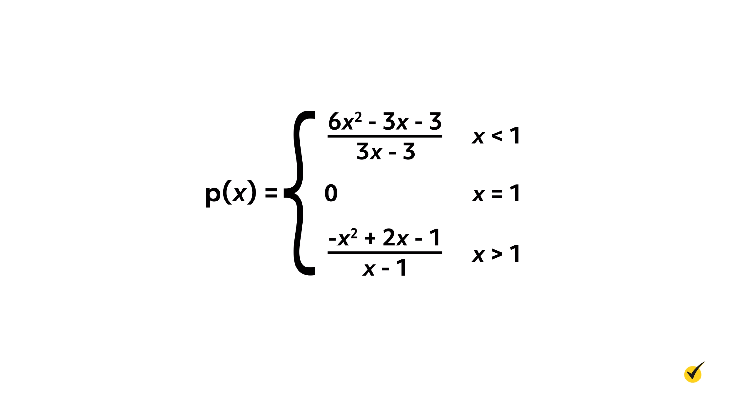
That last bit is really important! Sometimes you will encounter functions that do not approach the same value from both the left and the right. In these cases, the limit does not exist. For example, consider piecewise functions, which act differently along different areas of the domain, such as the function \(p(x)\).
\(p(x)\) is shown on this graph:
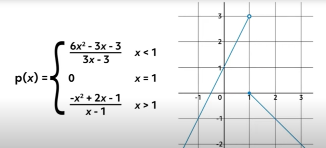
It is defined such that to the left of \(x=1\), it follows \(\frac{6x^{2}-3x-3}{3x-3}\), and to the right of \(x=1\) it follows \(\frac{-x^{2}+2x-1}{x-1}\). At the exact point \(x=1\), \(p(x)\) is defined such that it gives us 0. All of this means that we know exactly what \(p(x)\) is doing, across the entire domain.
However, if we were asked to find the \(\displaystyle \lim_{x\text{ }\rightarrow \text{ }1}\text{ }p(x)\), we would have to note the different behavior on the left and right sides of \(x=1\). On the left side, \(p(x)\) is approaching 3, but on the right side it is approaching 0. For this reason, even though we know how p behaves at the exact point \(x=1\), the \(\displaystyle \lim_{x\text{ }\rightarrow \text{ }1}\text{ }p(x)\) does not exist.
Mathematically, we express this left-and-right limit rule by saying, “the limit as \(x\) approaches a minus (that is, a from the left) of \(f(x)\), must equal the limit as \(x\) approaches a plus (a from the right) of \(f(x)\) in order for the limit to exist.”
Limits and Infinity
If we were to take the \(\displaystyle \lim_{x\text{ }\rightarrow \text{ }0}\frac{1}{x}\), we would see that on the right side, the function shoots upward toward infinity, and on the left side it dives downward toward negative infinity. Clearly, these are not the same value, so the limit does not exist.
We can, however, take the \(\displaystyle \lim_{x\text{ }\rightarrow \text{ }0}\left | \frac{1}{x} \right |\), because both sides will then behave similarly. For this limit, see how both sides shoot almost straight upward near \(x=0\). Whenever there is a vertical asymptote like this one, we say the limit tends toward infinity (or negative infinity whenever the function dives downward).
Now that we are talking about infinity, another important thing to note about limits is that we can take the limit of a function as \(x\rightarrow \infty\), or as \(x\rightarrow \text{ }- \infty\). In other words, we can observe how a function acts as \(x\) grows larger and larger without bound, as well as how a function acts as \(x\) grows more and more largely negative.
Let’s look at the function \(f(x)=\frac{1}{x}\) again, and see if we can determine this function’s limits as \(x\rightarrow + \text{ }\infty\), and then as \(x \rightarrow -\infty\).
First, how does \(f(x)\) behave as \(x \rightarrow + \text{ }\infty\)? Since \(\infty\) is not a real number, we can’t just substitute it into \(\frac{1}{x}\), but we can evaluate this limit by asking ourselves, “How does \(\frac{1}{x}\) behave as \(x\) grows larger and larger?”
We know that fractions with larger denominators are smaller in value than those with smaller denominators (for example, \(\frac{1}{3}\lt \frac{1}{2}\)). This means that as \(x\) grows larger and larger, the fraction \(\frac{1}{x}\) is shrinking. It always remains positive as long as \(x\) is positive, so although it never crosses 0, it does close in on 0 asymptotically. We also can observe this by looking at the graph of \(f(x)\).
The further right we look, the closer the line gets to the horizontal axis. Because of our knowledge of how fractions behave and because of what we see on the graph, we now know that the \(\displaystyle \lim_{x\text{ }\rightarrow \infty }\frac{1}{x}=\text{ }0\).
It may come as no surprise that we can find the \(\displaystyle \lim_{x\text{ }\rightarrow \text{ }-\infty }\frac{1}{x}\) in a similar fashion.
Again, larger denominators yield smaller values of fractions, so even though \(x\) is growing to larger and larger negative values, the fraction \(\frac{1}{x}\) is again getting closer and closer to 0, just from the negative side this time. We can check our intuition against the graph, which does in fact model this behavior.
The further left we look, the closer the line again gets to the horizontal axis.
Limits of Trigonometric Functions at Infinity
Let’s work one more example with limits at infinity.
As \(x\) grows larger and larger, how does the sine curve behave? Is there a single value it gets closer and closer to? Well, since the sine curve is an oscillating function, there is no single value it converges to. It follows the same wave over and over again, to infinity. Because of this:
Operations and Rules
Before we wrap up this video, I’m going to leave you with some useful operations.
If you ever need to find the limit of the sum or difference of two functions, you can find their limits individually and then add or subtract them appropriately.
Similarly, if you need to find the limit of two functions multiplied together or divided from each other, take their limits individually and then multiply or divide appropriately. We can express these properties mathematically.
\(\displaystyle \lim_{x\text{ }\rightarrow \text{ }a}\frac{f(x)}{g(x)}=\frac{\displaystyle \lim_{x\text{ }\rightarrow \text{ }a}f(x)}{\displaystyle \lim_{x\rightarrow \text{ }a}g(x)}\)
Note that for the division property, both \(g(x)\) and the \(\displaystyle \lim_{x\text{ }\rightarrow \text{ }a}g(x)\) must not be equal to 0. L’Hopital’s rule, where you take the derivative of the numerator and the denominator, may be necessary to simplify expressions given by the division property.
If you find yourself needing to take the limit of a function raised to some power, start by finding the limit of the function itself, then applying the power afterward. Mathematically, this power property can be stated as:
In the same vein, this also provides us with a root property. The limit of a root of the function \(f\) is equal to the same root over the limit of \(f\).
Finally, we also have a scalar multiple property of limits. By this, we mean that the limit of a function multiplied by a scalar constant is equal to the constant times the limit of the function.
Let’s quickly recap all that we’ve learned.
- Limits help us determine how functions act near certain points, but not necessarily what the functions are actually equal to at those points.
- We can evaluate limits by building tables or by observing the graphs of functions.
- A function must approach the same value from the left and right sides in order for the limit to exist.
- We can take the limit of a function at \(\infty\) by seeing how the function behaves as \(x\) grows larger and larger.
- Oscillating functions like the sine wave do not converge to any one point at \(\infty\), so that limit does not exist.
- And finally, many operations are preserved in limits, including addition and subtraction, multiplication and division, and powers and roots.
I hope this video has been helpful to you as an overview of limits and how we use them.
Thanks for watching, and happy studying!