

Hi, and welcome to this video about the trapezoid rule!
From Riemann Sums to the Trapezoid Rule
Left and Right Riemann Sum Review
Consider the problem of finding the area beneath a curve. By now, you probably should be familiar with the method of using Riemann sums, where we partition the domain of the curve into segments of equal width and then draw rectangles up to the height of the curve. The sum of the areas of these rectangles gives us an estimate of the area beneath the curve, and the more rectangles we use, the narrower the rectangles become, and the closer our estimation is to the true answer.
You should already know about left and right Riemann sums, but today we will discuss a new method, the trapezoid rule, but today we will discuss a new method, the trapezoid rule, that will give us greater accuracy without having to increase the number of partitions used.
Let’s begin with an example: use the left and right Riemann sum methods to generate estimates for the area beneath the curve \(y=x^{2}+1\) on the domain \(x=\left [ 0,3\right ]\) using step size (or width) \(s=1\).
Our curve, \(y=x^{2}+1\), looks like this on a graph:

Since we are considering the domain \(x\) from 0 to 3 with step size, or width, of 1, we will be paying special attention to the points on the curve where \(x=0\),\(x=1\), \(x=2\), and \(x=3\). These points will help us construct three rectangles.

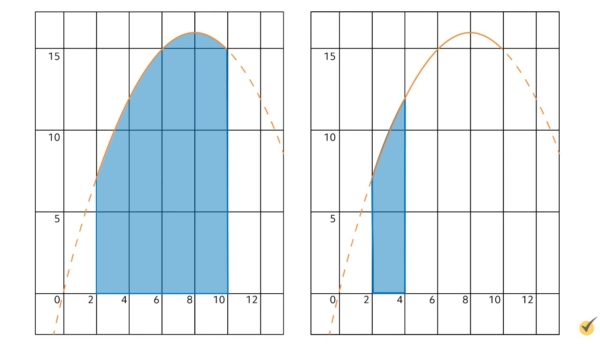
Now, for the left Riemann sum, the height of each rectangle will be equal to the height of the point of the curve at the leftmost point of that rectangle. The first rectangle, whose left edge lies on \(x=0\), will have height equal to \(y(0)=0^{2}+1=1\). The second rectangle will have height equal to \(y(1)=2\), and the third rectangle will have height equal to \(y(2)=5\). Again, these rectangles will look like this:

Alternatively, the rectangles for the right Riemann sum are constructed so that their heights are equal to the height of the curve at their rightmost point. So then the first rectangle has height \(y(1)=2\), the second has height \(y(2)=5\), and the third has height \(y(3)=10\). These rectangles look like this:

Notice that in both the left and right Riemann methods, our rectangles each cover either too much or too little area. The red rectangles, representing the left sum, leave a significant area unaccounted for, while the blue rectangles, which represent the right sum, count far too much.

Why Trapezoids Improve the Estimate
To get a better approximation for the area beneath our curve, we can narrow the step size and construct more, narrower rectangles. However, this can be very time consuming. And that’s where our trapezoid rule comes in! What if, instead of measuring area with rectangles, we “connect the dots” between steps to form trapezoids?
Continuing with our initial function and domain, this is what those trapezoids would look like:

What a drastic improvement from the left and right Riemann sums! To show just how major it actually is, note that the left Riemann sum with three rectangles estimated that the area beneath our curve was near 8. The right Riemann sum with three rectangles estimated that the area was near 17. The true value of the area beneath the curve is equal to 12, and in the same three partitions, the trapezoid rule estimated that the area was near 12.5, with an error of only 0.5!
| Method | Estimation of Area | Error |
|---|---|---|
| Left Riemann Sum | 8 | 4.0 |
| Right Riemann Sum | 17 | 5.0 |
| Trapezoid Rule | 12.5 | 0.5 |
Using the Trapezoid Rule
Now that we can clearly see how effective the trapezoid rule is, let’s discuss how we actually form these trapezoids and how to compute the sum of their areas.
Example: Four Trapezoids on \([2,10]\)
For this example, consider the function \(y(x)=-\frac{1}{4}x^{2}+4x\) on the domain \(x=\left [ 2,10\right ]\) with four trapezoids and step size \(s=2\). So we’re going to write out all this information so that we don’t forget it.
Then, we said that our domain is from 2 to 10, and we’re going to write it in interval notation.
And then our trapezoids have a step size of \(s=2\).
So that we have an idea what we are working with, this is what our function looks like:
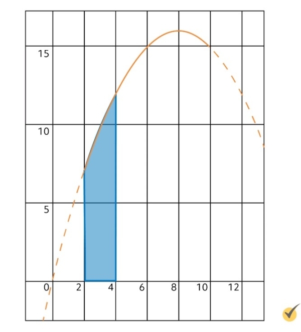
Since our step size is 2, each trapezoid’s base will have a width equal to 2, and we will be drawing our trapezoids between \(x=2\), \(x=4\), \(x=6\), \(x=8\), and \(x=10\). The first trapezoid will be between \(x=2\) and \(x=4\), so we need to find the value of the function at those points first.
So let’s find \(f(2\)). To find \(f(2)\), we plug in a 2 anywhere we see an \(x\), so we have:
So, \(f(2)=7\). Now, let’s find \(f(4)\).
So \(f(4)=12\).
The top, diagonal portion of the trapezoid can be drawn by connecting these two points with a straight line. With this information, we now know what our first trapezoid will look like.
The Trapezoid Area Formula
Remember from geometry that the area of a trapezoid can be found using the formula \(A=\frac{b_1+b_2}{2}\times \text{ h}\), where in this case, \(b_{1}\) is the length of the left side, \(b_{2}\) is the length of the right side, and \(h\) is the width of the base.
In these problems, \(h\) is equal to our step size \(s\). When we notice that the lengths of the left and right sides are just equal to the height of the curve at those points, we can rewrite this formula like this:
Here, \(x_{0}\) and \(x_{1}\) are the left and right endpoints of that trapezoid.
Now that we’ve got a formula, we can easily determine the areas of our trapezoids! For the first one, we plug in \(x_{0}=2\) and \(x_{1}=4\) to find its area. This is going to be the first area that we find, so we’re going to call it \(A_{1}\).
So, now we plug in our values. \(f(2)=7\), \(f(4)=12\), over 2, and we set our step size also to 2.
So, if we multiply, we can see that our 2s cancel out and we’re left with:
The second trapezoid starts at \(x=4\) and goes to \(x=6\), so we can plug those values into our formula. We already know that \(f(4)=12\), so we need to calculate \(f(6)\) before we can plug it into our formula for area.
Since \(f(6)=15\), we can find our second area.
Again, we can cancel out our dividing by 2 and multiplying by 2, and then we’re left with:
For the third trapezoid, we need to compute \(f(8)\).
Now, we find the area of the third trapezoid.
Again, our 2s will cancel out, and we’re left with:
We’ve got one last trapezoid to go. So, we need to compute \(f(10)\) to solve for that one.
So area of our fourth trapezoid, \(A_{4}\), will be equal to:
These 2s cancel each other out, and we’re left with:
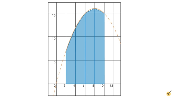
Our trapezoids for this example look like this:
Our estimate of the area beneath the curve from \(x=2\) to \(x=10\) using four partitions is then equal to the sum of these four areas:
So, let’s look at all these values and add them together.
The exact area beneath this curve is equal to 109.333.., so this is a very good estimate! For comparison, the left Riemann sum with four rectangles would have given us 100, and the right Riemann sum would have given us 116.
The Composite Trapezoid Rule Formula
Because we compute the values of each trapezoid using the same formula, we can write the following summation as a formula for the entire process:
In this formula, the subscripts simply denote which \(x\)-values are being dealt with, and these change from trapezoid to trapezoid along the way. The leftmost point of the domain is denoted by \(x_{0}\), and the rightmost point is denoted by \(x_{n}\), where \(n\) is the number of trapezoids.
Example: Three Trapezoids on \([0,1.5]\)
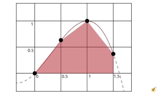
Let’s do one more example. Use the trapezoid rule to estimate the area beneath the function \(f(x)=-x^{3}+x^{2}+x\) on the domain \(x=0\) to \(x=1.5\) with step size \(s=0.5\) and three trapezoids.
So, we have our function:
Our domain is from, \(x=0\) to \(x=1.5\). So, if we write that in interval notation, that’ll look like this.
And then, our step size is:
To find the areas of each trapezoid, we will need the values of \(f(0)\),\(f(0.5)\),\(f(1)\), and \(f(1.5)\), so let’s go ahead and calculate those now.
\(f(0.5)=-(0.5 )^{3}+(0.5)^{2}\)\(\:=(-0.125)+0.25+0.5\)\(\:=0.625\)
\(f(1)=-(1)^{3}+(1)^{2}+(1)\)\(\:=-1+1+1=1\)
\(f(1.5)=-(1.5)^{3}+(1.5)^{2}\)\(+(1.5)\)\(\:=-3.375 +2.25 + 1.5\)\(\:=0.375\)
From these calculations, we can tell that the function goes up until it peaks, then starts coming down again, which is reflected in its graph:
Now, let’s start finding the areas of our trapezoids. The area of our first trapezoid, \(A_{1}\), is between \(x=0\) and \(x=0.5\), so let’s plug that into our formula.
Moving right along, let’s find the second trapezoid’s area.
And now, we can calculate the third and final trapezoid.
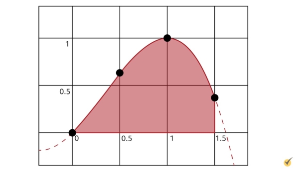
For this example, our trapezoids look like this:
To finish our estimation of the area beneath the curve, we simply add all our areas together.
This solution, like the other examples, is a good estimate! The true value of the area we are estimating is approximately 0.984. It is worth noting that accuracy can be improved for any and all of these methods by decreasing the step size and increasing the number of partitions, but clearly the trapezoid rule gives the best accuracy of these methods with the same number of steps.
I hope that this video has been helpful in shaping your understanding of the trapezoid rule and how to use it.
Thanks for watching, and happy studying!