Second Derivative Test

We already know that setting a function \(f(x)\) equal to zero and solving will give us the \(x\)-intercepts for that function. We also know that setting the derivative, \(f'(x)\), equal to zero and solving will give us the points where the function’s tangent line is horizontally flat.
\(f'(a)=0\rightarrow\) flat at \(a\)
What kind of information do we get from the second derivative, though? Let’s find out.
Let’s start this lesson with a couple definitions. In this graph, we can see a function with multiple “peaks” and “valleys”. Such points are generally called extrema.
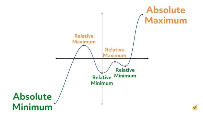
More specifically though, the peaks are called maximums, while the points at the bottoms of valleys are called minimums.
Moreover, the points on a graph which are the highest of all or lowest of all are called the absolute maximum and absolute minimum, respectively.
Minimums and maximums that are not absolute mins and maxes are called relative minimums and maximums.
Let’s take a moment to identify extrema in other graphs and label them accordingly.
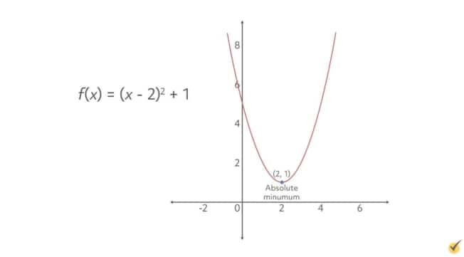
This function is one big valley, and we can easily spot that its vertex is here. This point is an extrema—specifically a minimum. Further, being that it is the lowest point in the entire graph, this is the absolute minimum. Let’s label it as such.
Okay, let’s look at another curve now.
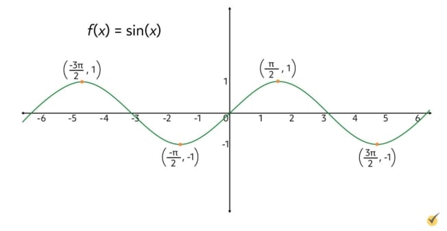
This familiar function is the sine curve, which has repeating peaks and valleys. Let’s mark the extrema now.
As we can see, the points with height 1 are maximums, while the points with height \(-1\) are minimums. Does this graph have any absolute maximums or minimums? Since each maximum has the same height, and since each minimum has the same height, the answer is no. There is no single point which is higher or lower than all other points on the sine curve. Each of the extrema on this graph is a relative maximum or minimum.
Recall from previous lessons that a critical point is a point \(x\) which causes the derivative, \(f'(x)\), to equal zero or be undefined. These critical points are helpful for locating extrema.
If we find the second derivative, though, and set it equal to zero, we find something called an inflection point. An inflection point is a point on a graph where the direction of curvature changes. Let’s look at this graph.
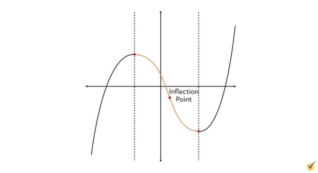
We already know that these two points are extrema; the first is a relative maximum, and the second is a relative minimum. At these two points, we know that the derivative of the function is equal to zero. To the left of the maximum, we can see that the function is increasing in height, meaning the derivative there is positive. To the right of the minimum, we see that the function is increasing again, meaning the derivative is, again, positive. What exactly is happening in between the extrema, though?
Since the function is decreasing on this interval, we know that the derivative is negative there. Notice the curviness of this section, though. In the left portion, the function starts out relatively flat and then “picks up speed” on its descent, causing the slope to become more and more negative. At a certain point though, this negativity begins to reverse, and the function eventually flattens out again just in time for the minimum. The point along the way where the slope begins to “change directions” and return towards being flat is called the inflection point. For this function, the inflection point is right around here:
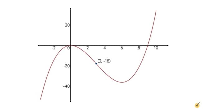
As I mentioned before, inflection points can also be found algebraically by setting the function’s second derivative equal to zero and solving. For example, we can find the inflection point for the function \(f(x)=\frac{1}{3}x^{3}-3x^{2}\) by finding the second derivative. So we’re gonna take the first derivative and we’ll have:
And then we’ll take the second derivative.
And then we can solve for where that equals zero.
\(6=2x\)
\(3=x\)
For this function, there is an inflection point at \(x=3\). We can find the \(y\)-coordinate of this point by evaluating \(f(3)\).
The graph of this function, including the inflection point, looks like this:
Finding inflection points is at the heart of what we call the “second derivative test.” Usually for these, in addition to locating inflection points, you’ll be asked to determine the function’s concavity by region of the graph.
When it comes to concavity, there are four categories that a region of a curve may fall into: increasing and concave up, increasing and concave down, decreasing and concave up, and decreasing and concave down. Here’s what I mean.
Let’s say a curve is increasing on a certain region of the graph. This part of the curve may look either like this or this.
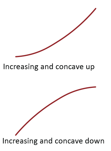
Notice that while both curves are increasing in height, the first curve’s slope is growing, while the second curve’s slope is tapering off and flattening out. For this reason, the first curve is classified as “increasing and concave up” while the second is “increasing and concave down.”
On the other hand, a curve which is decreasing in height may look either like this or this.
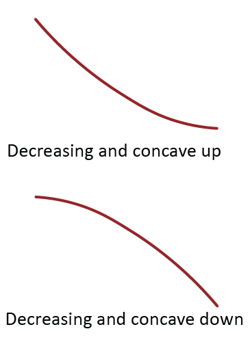
The first curve is classified as “decreasing and concave up” while the second is “decreasing and concave down.” A good way to remember these classifications is that you first want to determine whether the curve is increasing or decreasing in height. Then, you can determine whether it is concave up or down by checking whether the curve is “hugging” the area above it or below it respectively.
Another way of determining concavity, if you do not have a graph to look at, is by determining the signs of the first and second derivative. A positive first derivative corresponds to increasing height, while a negative first derivative implies that height is decreasing. The second derivative informs us about whether the curve is concave up or concave down in that region. A positive second derivative corresponds to concave up, while a negative second derivative corresponds to concave down.
| \(f'(x)\gt 0\) | \(f'(x)\lt 0\) | |
| \(f”(x)\gt 0\) | Increasing and concave up | Decreasing and concave up |
| \(f”(x)\lt 0\) | Increasing and concave down | Decreasing and concave down |
To determine on what region a curve is a particular concavity, it is helpful to locate critical points and inflection points. These are points at which concavity and directions change.
Let’s try putting all of this information to work now in a second derivative test. For the function \(g(x)=\frac{1}{3}x^{3}+2x^{2}-5x\), locate any critical points and label extrema as absolute or relative minimums or maximums. Then determine where any inflection points lie. Finally, determine the concavity of the function by region.
Although this problem is asking for a lot of information, we have the tools to work through it with relative ease. First, we need to know where any critical points are. To do this, we need to find \(g'(x)\), set it equal to zero, and solve. So if we take the first derivative, we’ll get:
If we set this equal to zero, we’ll have \(0=x^{2}+4x-5\). Then to find the solutions, we can factor this expression, and we’ll get:
And we can set both of these equal to zero to solve, so we’ll have:
| \(x+5=0\) | \(x-1=0\) |
| \(x=-5\) | \(x=1\) |
So there are critical points at \(x=-5\) and \(x=1\). We can get the ordered pairs for these two points by evaluating \(g(1)\) and \(g(-5)\). So, let’s do that now.
\(g(1)=\frac{1}{3}(1)^{3}+2(1)^{2}-5(1)\)\(=-\frac{8}{3}\)
The critical points for this function are then at \((1,-\frac{8}{3})\) and \(-5,\frac{100}{3}\). The next thing we need to determine is where extrema are and how they are labeled. Since extrema occur where the derivative equals zero, our two critical points are the only extrema for this problem. To determine whether they are maximums or minimums, we can check the slope of the function in areas surrounding these points.
To find the slope to the left of \(–5\), let’s choose a number smaller than \(–5\) and plug it into the function \(g'(x)\). \(–6\) will do just fine. The slope at \(x=-6\) is:
So the slope to the left of \(-5\) is positive. What about the slope between \(-5\) and 1? Let’s check at one of the points between, such as 0.
So the slope between \(x=-5\) and \(x=1\) is negative. Let’s check the slope now to the right of positive 1, using the point positive 2.
So the slope to the right of \(x=1\) is positive.
| \(x\lt -5\) | \(g’x\gt 0\) |
| \(-5\lt x\lt 1\) | \(g’x\lt 0\) |
| \(x\gt 1\) | \(g’x\gt 0\) |
This information suggests that the critical point at \(x=-5\) is a maximum and that the critical point at \(x=1\) is a minimum. Because the function goes up and down further than the critical points, though, they are not absolute extrema, and are rather relative extrema.
\((1,-\frac{8}{3})\) is a relative minimum
Our next task is locating any inflection points. To do this, we need to take the second derivative and find where it equals zero. Since we already know \(g'(x)=x^{2}+4x-5\), we can now find the second derivative.
Where does \(2x+4\) equal zero? We can find out by quickly solving.
\(-4=2x\)
\(-2=x\)
This means that the inflection point for this function occurs when \(x=-2\). To get the \(y\)-coordinate for the ordered pair, we can evaluate g at \(-2\).
The inflection point occurs at \((-2,\frac{46}{3})\).
The final task in this problem is determining the concavity of \(g\) over its different regions. Based on our work locating critical points and the inflection point, we will have to determine concavity for the following regions: points to the left of \(–5\), points between \(–5\) and \(–2\), points between \(–2\) and \(+1\), and points greater than 1.
| \(x\lt -5\) | |
| \(-5\lt x\lt -2\) | |
| \(-2\lt x\lt 1\) | |
| \(x\gt 1\) |
In order to properly determine these concavities, let’s refer back to our guide from earlier:
| \(f'(x)\gt 0\) | \(f'(x)\lt 0\) | |
| \(f”(x)\gt 0\) | Increasing and concave up | Decreasing and concave up |
| \(f”(x)\lt 0\) | Increasing and concave down | Decreasing and concave down |
We have already determined where the first derivative is positive and negative, so in order to determine concavity, we just need to find where the second derivative is positive and negative. Let’s check one point to the left of \(–2\) and one to the right.
For the left, let’s use \(–3\).
So the second derivative is negative to the left of \(x=-2\). To check a point to the right of \(–2\), let’s use 0.
This is positive, so the second derivative is positive to the right of \(x=-2\).
Now, onto pairing each type of concavity with the different regions.
Because we said the function has a positive first derivative to the left of \(–5\) and to the right of positive 1, those regions are going to be classified as “increasing.” However, the region to the left of \(–5\) has a negative second derivative, making it concave down, while the region to the right of \(+1\) has a positive second derivative making it concave up.
| \(x\lt -5\) | Increasing and concave down |
| \(-5\lt x\lt -2\) | |
| \(-2\lt x\lt 1\) | |
| \(x\gt 1\) | Increasing and concave up |
The remaining regions between \(–5\) and \(+1\) both have negative values for the first derivative, making them “decreasing.” The region between \(–5\) and \(–2\) has a negative second derivative, making it concave down. On the other hand, the region between \(–2\) and \(+1\) has a positive second derivative, making it concave up.
| \(x\lt -5\) | Increasing and concave down |
| \(-5\lt x\lt -2\) | Decreasing and concave down |
| \(-2\lt x\lt 1\) | Decreasing and concave up |
| \(x\gt 1\) | Increasing and concave up |
At last, we have completed all parts of the second derivative test. We located critical points, labeled extrema, found an inflection point, and determined concavity by region. While this process can seem lengthy, as with all things, it gets easier with practice. I hope you’ll go try some problems on your own now!
Thanks for watching, and happy studying!