Population Growth

Hi, and welcome to this video about population growth! Today, we’re going to cover the unique features of exponential functions and how they are used to model population growth. I’m going to give you a few practice problems later on, so go ahead and make sure you’ve got a calculator handy if you want to try to solve them yourself. Let’s get started!

Before we dive in, let’s remind ourselves of the basics of functions. In simple terms, functions provide the rules on how to mathematically adjust “input” to get “output.” Here’s a simple linear equation:

These rules arrive at the “output” by multiplying the “input” by the constant, \(m\), and adding the value of \(b\). As you know, the graph of any linear function is a line that increases at a constant rate when the slope, \(m\), is positive. These functions are helpful to visualize data that is linear in nature.

In contrast, exponential functions, which are the focus of this video, are used as models for data that increase rapidly over time. This is known as a pattern of exponential growth. An exponential function is written in the form, \(f(x)=ab^{x}\), where:

Because the growth factor, \(b\), is being raised to a power that is a variable, \(x\), the rate of change in an exponential function is not constant.

The graph here shows the difference between the steady increase of a linear function and the extreme, rapid increase of a function showing exponential growth over time:

Now that we’ve seen the shape of a function that shows exponential growth, let’s look at a few ways this relates to population growth.

Population growth is an interesting concept from many different perspectives. For example, biologists can study the growth patterns of living organisms based on reproductive facts and environmental needs of the species. Another application would be global health professionals and conservationists who investigate the exponential growth that our world population has experienced.

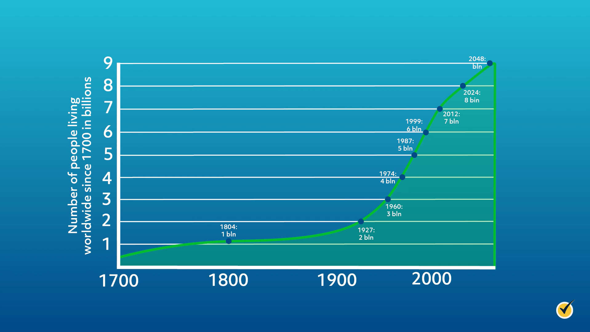
As you can see, our planet has sustained an exponential increase of approximately 6.6 billion people since 1800, with most of that growth occurring during the 20th century!

When dealing with “natural” population growth models, you will notice that the notation is slightly different from a standard math exponential function.

A population model requires the use of the irrational number \(e\), which has an approximate value of 2.71828, as the base. This base is then raised to a power that reflects the growth rate, \(r\), and a unit of time, \(t\). This is the general form of an exponential population growth model.

It is also important to note that this type of growth model is only effective to use for short cycles of time, as true populations are typically limited by external factors that impact growth such as food supply and mortality. Logistic population growth models are more appropriate to use when there are known limitations on growth capacity.

Let’s apply the exponential population growth formula with a few practice problems:

Let’s assume that we’re inspecting a certain bacteria that grows exponentially. If there were 100 bacteria present in a lab sample at 1pm and the growth rate is known to be 2.5% per hour, calculate the number of bacteria that was observed at 4pm.

Our first step is to identify the components of the formula. Here’s what we know:

The initial population of the bacteria is 100.

The rate of growth is 2.5% per hour, which converts to a decimal value of 0.025.

The amount of time that elapsed in the lab is 3 hours.

 
For \(e\), you can use the approximate value of 2.71828 if you do not have a scientific calculator.

We need to use this information to determine the final population, \(P\).

Using a calculator to compute the final population, \( P=100e^{(0.025\cdot 3)}\), we get that

In words, the bacteria in the sample grew from 100 to approximately 108 in 3 hours.

Okay, let’s look at another example. This time, I want you to try to work it out on your own before I tell you the answer.

Our world population totaled 7,631,091,040 at the end of 2018. This reflects a 1.1% increase over the prior year. To practice using the population growth formula, use this information to estimate the world population in the year 2019.

Pause the video if you want to try it out on your own.

So, let’s look at the information we know and plug it all into our equation.

 
So we have our initial world population

 
The rate of growth is 1.1%, which converts to a decimal value of 0.011.

 
The number of years from 2018 to 2019 is 1.

 
An approximate value of \(e=2.71828\) can be used.

Using this information and a calculator, it is estimated that the world population was approximately 7.716 billion at the end of 2019.

The actual population at the end of 2019 was about 7.714 billion people, which reflects roughly 2 million fewer people from what your estimate should have been!

So, we’ve looked at a couple of examples that require you to find the final population. But what if you were already given the final population and asked to find the initial population? Let’s look at an example:

As of 2020, the population of Africa was approximately 1.341 billion. The annual growth rate is calculated at 2.49%. Use the population growth formula to determine the African population at this time in 2019.

Here’s what we know. The final population of Africa is approximately 1.341 billion.

The rate of growth is 2.49%, which converts to a decimal value of 0.0249.

The number of years from 2019 to 2020 is 1.

 
An approximate value of \(e=2.71828\) can be used.

We are asked to determine the initial population, \(P_{0}\). First, use a calculator to determine the constant value that is multiplied by \(P_{0}\), \(e^{0.0249}\). So now we know that:

Now, solve for \(P_{0}\) by dividing both sides of the equation by 1.0252.

In this case, the “original” population represents the year 2019. Our calculation shows that value to be about 1.308 billion people.

Here is another example:

The United Nations estimated that the United States population will be 331,002,651 by mid-year 2020, and the expected growth rate is estimated at 0.59%. Use this information to determine the US population at mid-year 2022. (Assume that the growth rate is the same between 2020-2021 and 2021-2022.)

Pause the video now if you’d like to try this one on your own.

Ok, so here’s what we know:

The US population is estimated to be about 331 million at mid-year, 2020.

The rate of growth is 0.59%, which converts to a decimal value of 0.0059.

The number of years from 2020 to 2022 is 2.

An approximate value of \(e=2.71828\) can be used.

We are asked to determine population, \(P\), in mid-year 2022. Since we’ve substituted the known values in our equation, we can use our calculator to find our final answer, which is approximately 335 million.

We can also use this formula to solve for \(t\), the number of years it takes for the original population to grow to the final population. When we solve for any variable, we use algebraic steps to isolate it in order to determine its value. However, in this case, the variable for time is in the exponent of the formula. How can we get to it in order to find its value?

This can be done by using the inverse function that “undoes” the work of the exponential function. It is called the natural log, and is notated as \(ln\). Consider that the exponential function, \(f(x)=e^{x}\), takes in the input, \(x\), and results in the output, \(e^{x}\). Applying the natural log, \(ln\), to this output results in the original input, \(x\). This identity is shown as \(ln(e^{x})=x\).

If we want to solve for the variable \(t\) in a population formula, it is as simple as hitting the natural log key on your calculator and continuing with a few additional algebraic steps.

Let’s try one last example to practice using the natural log.

The current population of Iceland is approximately 341,400 people. The annual growth rate of the population is approximately 0.65%. Assume that this rate of growth will continue in the future. How many years will it take for the population to reach 400,000?

Well, we could simply multiply the current population by the annual growth rate for as many times as it takes to get to 400,000, but solving the exponential equation for \(t\) is a lot more efficient and precise..

As before, let’s list what we know:

Iceland’s population is estimated to be 341,400.

The rate of growth is 0.65%, which converts to a decimal value of 0.0065.

The population that we are targeting is 400,000.

An approximate value of \(e=2.71828 \) can be used.

As you can see, the unknown in this equation is time. We have to use algebraic steps and the natural log function to solve for the amount of time it will take for the population to be equal to 400,000.

Step 1: Divide both sides of the equation by \(P_{0}\), which will leave an exponential expression on the right.

Note that we will be rounding our answers from the calculator to four decimal places to illustrate this example, but leaving the values in the calculator unrounded gives a more accurate answer.

We are now ready to apply the natural log to the exponential expression on the right side of the equation so we can do the work to solve for \(t\). However, as we know from solving equations, if we perform an operation on one side of the equal sign, you must do the same on the other side to maintain balance.

Here is what taking the natural log of both sides looks like. Step 2:

As mentioned, there is a key on your calculator to determine the value of \(ln(1.1716)\). Simply hit the \(ln\) key, and a parenthesis will appear. Enter 1.1716, and close the parentheses. Next, hit enter for a value of 0.1584. On the right side, the natural log “undoes” the exponential function, leaving the expression in the exponent, \(0.0065\cdot t\).

Now, the \(t\)-variable can be solved for by dividing both sides of the equation by 0.0065, as follows. Step 3:

We now know that it will take about 24 and a half years for the population of Iceland to reach 400,000 people.

That’s all for this review! Now that we’ve worked through some examples, you should better understand the features of exponential functions and how they are used to model population growth.

Thanks for watching, and happy studying!

Population Growth Practice Questions