Midpoint Rule

Hi, and welcome to this video about the midpoint rule! In this video, we will explore what the midpoint rule is, what it’s used for, and walk through a couple of examples of how to use it. Let’s get started!

Analyzing Riemann Sums

One of the quickest ways to estimate the area under a curve is to use a Riemann sum, which essentially involves adding up a series of geometric shapes of equal width. There are different types of Riemann sums – you probably have experience with right and left rectangles. With all Riemann sums, the more shapes we add over an interval, the more accurate our estimate is.

Here, we have the function \(f(x)=x^{3}-6x+8\) with the area under its curve being measured with a right Riemann sum over the interval [-2,3] using 5 rectangles of width 1:

Notice that, when the graph is decreasing, the rectangles give an underestimate and when the graph is increasing, they give an overestimate. The steeper the sections of the graph, the more these trends are exacerbated.

Here’s the same area estimate using a left Riemann sum:

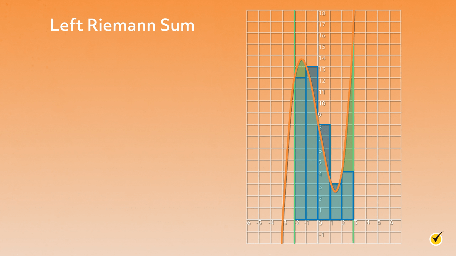
Notice the opposite trends are true: decreasing sections give an overestimate and increasing sections give an underestimate.

Which brings us to the midpoint rule.

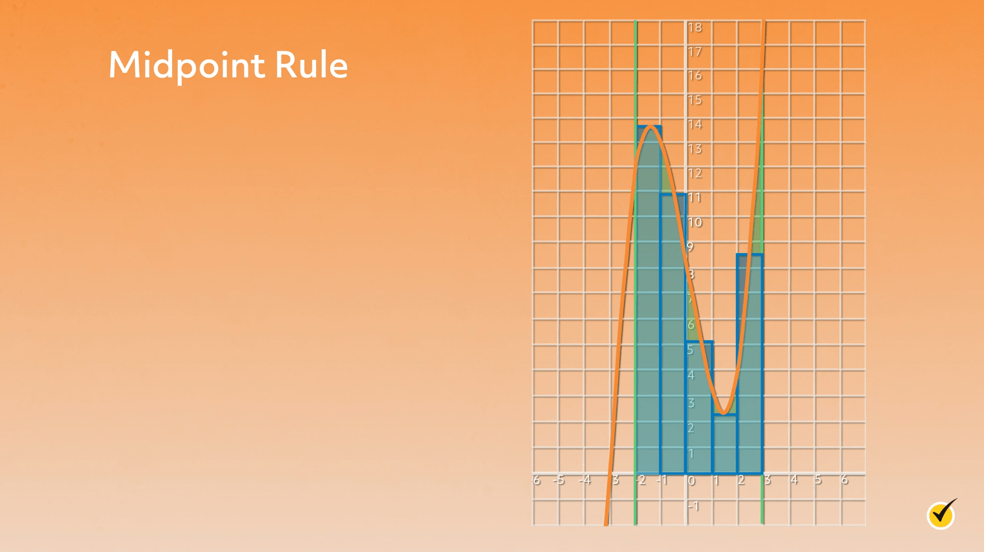
Again, same function, same estimate. But the rectangles are a little bit different:

Recall that with a right Riemann sum, the height of the rectangle is the height of their right edges, and with a left Riemann, the height is that of their left edges. With the midpoint rule, a third type of Riemann sum, the rectangle height is the height of the midpoint of the top edge. On the graph, you can see the result is kind of an “in between” estimate – each rectangle has a bit of over- and a bit of under-estimation. If we were to calculate all three sums, which we will do shortly, the midpoint rule would give us an estimate somewhere between the right and the left. Though still just an estimate, the midpoint rule is typically more accurate than the right and left Riemann sums.

Here’s an example of the rule being used in a math problem:

Estimate the area under the curve \(f(x)=x^{3}-6x+8\) over the interval [-2,3] with 5 rectangles using the midpoint rule.

When this rule is specified in a problem like this, it sounds pretty much like the other two Riemann sums. As with the other methods, the trick is figuring out where to measure the height of each rectangle.

Remember, the area of a rectangle is \(w\times h\), and we’re going to add a bunch of them, so the general idea is the same as before:

More formally, the rule looks like this.

This is saying that the width of each rectangle is determined by taking the range of our interval (\(b-a\)) and dividing it by the number of rectangles we want to use (\(n\)). The more formal formula for finding area using midpoint looks like this:

Remember, \(a\) and \(b\) are the endpoints of the interval, and \(n\) is the number of rectangles.

Let’s take a minute to see how this applies to our practice problem.

\(a=-2\), \(b=3\), because those are the endpoints of our interval. \(n=5\) because that’s the number of rectangles we want to use. And \(\Delta x=1\), meaning that each rectangle is going to have a width of 1.

Now for the heights. The formula is telling us where to measure, we just need to put in some numbers.

So \(f(a+\frac{\Delta x}{2})\) is really just telling us to start by measuring \(f(-2+\frac{1}{2}\). Which is \(f(-1.5)\).

It’s literally telling us “measure the height at the left endpoint + half of a width.” The rest of the heights are \(\Delta x\) away, so we measure \(f(-0.5)\), \(f(0.5)\), \(f(1.5)\), and \(f(2.5)\).

Using the formula, the area looks like this:

A diagram can help in figuring out the calculation as well.

The area estimate ends up being this:

So the area using the midpoint is equal to 40.625.

For a quick comparison, the right Riemann sum is 45 and the left is 40. Notice how the midpoint estimate falls between, but not directly in the middle of, the other two estimates.

Let’s practice a couple!

1. Estimate the area under the curve \(f(x)=x^{2}+2\) over the interval [-1,2] with 6 rectangles using the midpoint rule.

The first thing we need to do is figure out our \(\Delta x\). So \(\Delta x\) is equal to our \(b-a\), so 2-(-1), over \(n\), which is the number of rectangles we want, so 6.

So 2-(-1) turns into 2+1, which is 3.

So the width of each rectangle is \(\frac{1}{2}\).

We need to measure the first height at half the width of rectangle 1. So, the first height will be:

So our entire approximation is:

Which, when we plug in our values, gives us this:

 
So the entire approximation is 8.9375. Let’s try another one!

2. Estimate the area under the curve \(f(x)=sinx\) over the interval [0,\(\Pi \)] with 4 rectangles using the midpoint rule.

The first thing we need to do is figure out our \(\Delta x\). So \(\Delta x\) is equal to \(b-a\), so \(\Pi -4\), over \(n\), the number of rectangles.

We need to measure the first height at half the width of rectangle 1. So, the first height will be:

After that, each height measurement is \(\Delta x\) away. So our entire approximation looks like this:

So our approximation is approximately equal to 2.05.

I hope that this video increased your knowledge about Riemann sums and helps as you estimate areas under curves!

Thanks for watching, and happy studying!