

Introduction to the Mean Value Theorem
Picture this: You drive through a tollbooth at the start of a 20-mile stretch of road at 12:30 pm. The speed limit over the entire section is 60 miles per hour. You exit through the tollbooth on the other side at 12:48 pm only to find a police officer waiting to give you a speeding ticket.
How did the officer know you were speeding without shooting your car with their radar gun? Calculus, of course!
Since the speed limit is 60 miles per hour, the fastest you can legally go is one mile per minute (60 miles in 60 minutes). So, it should have taken at least 20 minutes to make it to the other side (you can go slower). But you arrive in 18 minutes, so at some point you must have gone faster than 60 miles per hour. No radar gun needed.
The police officer applied the mean value theorem, which says for a continuous, differentiable function over a closed interval, at some point the instantaneous rate of change equals the average rate of change over the interval.
Formally stated, the theorem says:
If \(f\) is continuous over \([a,b]\) and differentiable over \((a,b)\), then there is a \(c\) in \((a,b)\) such that \(f^{‘}\left ( c \right )=\large{\frac{f\left ( b \right )-f\left ( a \right )}{b-a}}\).
The police officer knew that if your average rate of change was 20 miles per 18 minutes, or 1.1 miles per minute, at some instant on your trip, you must have traveled 1.1 miles per minute (speeding).
Graphing the Mean Value Theorem
Let’s explore the mean value theorem graphically using the points \((-2, 1)\) and \((4, 4)\). Connecting the points with a linear function clearly demonstrates the mean value theorem, since all points have an instantaneous rate of change of \(\frac{1}{2}\), which is the average rate of change over the interval:

What if a curved function goes through those points? On the interval \((-2, 4)\), there must be at least one tangent line that is parallel to the secant line. Recall that a secant line is a straight line that intersects a curve in at least two different points.
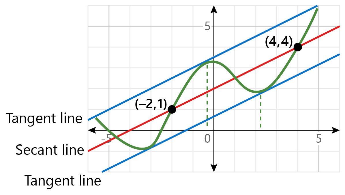
In this case, there are two tangent lines that are parallel to the secant line. You can imagine how the theorem would hold for functions of many different shapes.
Rolle’s Theorem
What if the endpoints of the interval are the same height? In the case of \(f(x)=1\) over the interval \([-2, 2]\), the average rate of change is zero, since there is no change in height. What about a non-linear function that passes through those same points?
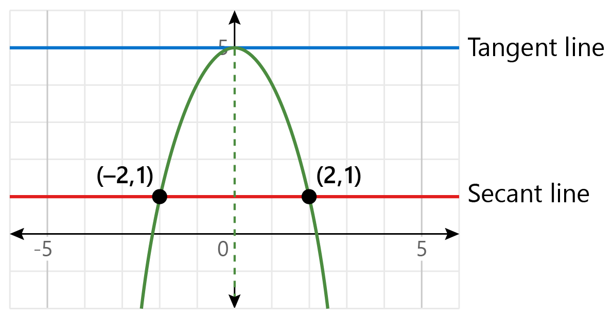
The function \(f(x)=-x^{2}+5\) passes through those points and there is a \(c\) such that \({f}'(c)=0\).
This “zero-slope secant line” scenario actually demonstrates Rolle’s theorem, which says if a continuous, differentiable function’s average rate of change over a closed interval is zero, then at some point in the interval the instantaneous rate of change must be zero.
Formally stated, here’s Rolle’s theorem:
Applying the Mean Value Theorem
Here’s what these theorems often look like in practice.
Let’s take a look at this function:
Before we begin, first note that since \(f(x)\) is a polynomial function, it satisfies the conditions of continuity and differentiability in both theorems, since it is continuous and differentiable everywhere. There are times where functions will not satisfy these conditions, so be sure to verify them!
Finding \(c\) with Rolle’s Theorem
What value(s) of \(c\) satisfy Rolle’s theorem over the interval \([-1,3]\)?
To use Rolle’s theorem, \(f(a)\) must equal \(f(b)\). So we’ll take \(f(-1)\) and plug it into our equation:
And this must equal our other end, so now let’s plug in \(f(3)\).
Since this is true, there must be a point \(c\) where the derivative also equals 0. So we’re gonna take the derivative of our function, we have:
So now we want to find where it equals 0. So, remember, we’re looking for the point \(c\), so we’re gonna put \(c\) in the place of \(x\).
Add 2 to both sides.
And then divide by 2 on both sides. So:
In this case, Rolle’s theorem and the mean value theorem can be interchanged.
Here’s the solution using the mean value theorem. So the mean value theorem says that \(\frac{f(b)-f(a)}{b-a}\) will give us our point where the derivative equals 0.
So \(f(b)=f(3)\).
According to the mean value theorem, there must be a place where the derivative equals 0. So again, we’re gonna take the derivative of this function.
And since there must be a place where it equals 0, do:
Add 2 to both sides.
Divide by 2 on both sides.
See, we get the same result either way, whether we use Rolle’s theorem or mean value theorem.
Finding \(c\) with the Mean Value Theorem
What values of \(c\) satisfy the mean value theorem over the interval \([-1,4]\)?
To use the mean value theorem, first find the slope of the secant line:
So first, let’s find \(f(4)\).
And then:
So now we can go back up here and plug these values in. So \(f(4)=2\), \(f(1)=-3\), so:
At some point in the interval, there is a tangent line with a slope of 1. So we’re gonna take the derivative of our function:
And at some point it must equal 1, so:
Add 2 to both sides.
And divide by 2 on both sides. So:
For which value of \(b\) in the interval \([-2,b]\) is the mean value theorem satisfied at \(c=0\)?
If the mean value theorem is satisfied, then the slope of the tangent line at \(c=0\) is the same as the slope of the secant line connecting the endpoints of the interval.
Let’s find the slope of the tangent line. Take the derivative of our function.
And then plug in 0 to find our derivative at \(x=0\).
The slope of the tangent line equals the slope of the secant line. So we’re gonna take this −2 and set that equal to:
\(-2=\dfrac{f(b)-f(-2)}{b-(-2)}\)
\(-2=\dfrac{(b^{2}-2b-6)-((-2)^{2}-2(-2)-6)}{b+2}\)
\(-2=\dfrac{b^{2}-2b-6-(2)}{b+2}\)
\(-2=\dfrac{b^{2}-2b-8}{b+2}\)
Then, if we factor out our numerator, we get (our \(b\)’s multiply together to get \(b^{2}\), −8 comes from −4 and +2):
Our \(b+2\)’s cancel out and we’re left with:
Add 4 to both sides, and we get:
Now let’s take a look at a place where we might have gotten a little tripped up. So let’s take a look at this step right here:
What if we multiplied \((b+2)\times 2\) and solved from there?
So if we distribute our −2, we get:
Add \(2b\) to both sides.
Add 8 to both sides.
And take the square root of both sides. That gives us:
Now, there’s a slight difference between our two answers. This answer (\(b=2\)) only gives us positive 2, and this answer (\(b=\pm 2\)) includes negative 2. We can’t include −2 because, if we look back, we have \(b+2\) in the denominator, so if we plug in −2, we’ll get a 0 in the denominator, which means that it’s undefined.
So even though we found two solutions this way, we know that there’s really only one solution that we’re looking for. There are a couple other reasons this is true. Negative 2 must lie in the open interval we’re considering, but \((-2,-2)\) is actually empty, and another reason is that since \(f(x)\) is quadratic, there’s only one turning point. There can be two \(c\) values with two or more turning points. It’s the same reason only one \(c\)-value was located in parts \(a\) and \(b\).
That’s it for the mean value theorem! I hope that this video helped with your understanding of this oh-so-important finding. You’ll see that it pops up in various places as you discover more calculus! I hope this video was helpful. Thanks for watching, and happy studying!