Matrices: Data Systems

A matrix is commonly defined as a rectangular array of numbers, symbols, or expressions arranged in rows and columns.

Matrices can be added, subtracted and multiplied and they can be manipulated in order to discern certain characteristics. However, they can also be representative of data and used in linear algebra applications.

Data Tables

A common representation of matrices is that of data tables. Suppose the owner of a burger chain wants to see cumulative data from three locations. Matrices could be used like this:

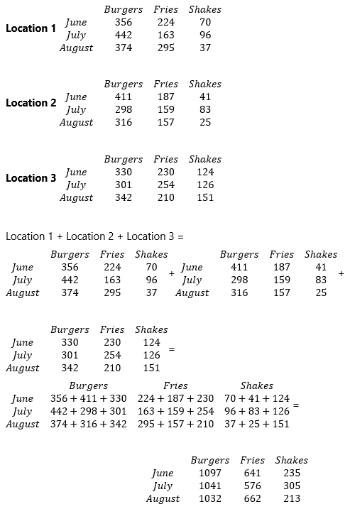
Since the dimensions of all three matrices are equal and the data in each corresponding entry represents the same quantity, i.e., the data in the row 1 column 1 entry is always June burgers, etc., these matrices can be added or subtracted as needed.

Solving Systems of Equations

Matrices can also be used to solve systems of linear equations. This method is parallel to the classic elimination method. Using that method, we can add equations together and multiply equations by scalars in order to isolate and solve for the different variables.

If this sounds familiar, it should, because those are also the legal row operations when working with matrices.

Let’s look at the steps involved, then we’ll look at a system in action.

1. For all equations in the system, put the terms in the same variable order (for example $x$, $y$, $z$)
2. Create a matrix using just the coefficients of the terms in the equations in the system. Put a 0 placeholder where variables don’t exist in an equation.
3. Augment the matrix with a constant matrix comprised of the solutions to the equations in the system.
4. Use row operations to get the matrix into reduced row echelon form.
5. Read off the solutions.

Here we go! Let’s solve this system:

The terms are in the same variable order, so let’s create the coefficient matrix:

Since an $x$-term is missing from the second equation, a zero is put into the row 2 column 1 position.

Now for the augmented matrix:

 
The vertical line inside the matrix is often used to show augmentation. When augmenting with a vector composed of the solutions to the equations in the system, it’s also a nice equal sign placeholder.

Now it’s time to row reduce.

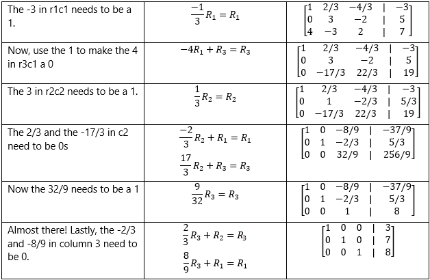
Now that our matrix is fully row reduced, all we need to do is read off the numbers. The matrix now gives us this:

The solution to the system might be written as (3,7,8).

Note that you don’t necessarily need to do the full row reduction in order to solve the system. For example, in the second to last step, the matrix says that:

 
Knowing the value of $z$ lets you substitute it into the other equations to figure out the values of $x$ and $y$.

The example system is an independent system because there is only one solution. Matrices can show dependent systems (infinite solutions, i.e. the same line) and inconsistent systems (no solution) as well.

If you are row reducing a matrix representing a system and create a zero row, then you have a dependent matrix. This is comparable to using substitution or elimination and ending up with $0=0$.

If you are row reducing a matrix representing a system and you create a zero row that has a nonzero number as the last entry, then you have an inconsistent matrix. This is comparable to using substitution or elimination and ending up with 0=some number.

Thanks for watching, and happy studying!

Matrix Practice Questions