Left and Right Riemann Sums

In geometry, we learned how to find the area of many shapes including rectangles, circles, triangles, and trapezoids. Each of these shapes has defined formulas to help us determine their areas, usually based on parameters like their height, length, or radius. But what if we wanted to determine the area lying beneath a curve?
In this video, we are going to talk about a method called Riemann sums for approximating areas like these.
Let’s take a look at that curve again. We haven’t yet gone over a well-defined method of determining the exact area beneath it, but we can start to get an idea of what the true area is close to by drawing in rectangles on the graph, like this:
Here, we have drawn rectangles of equal width (in this case, their widths are one unit wide), where each rectangle is as tall as the height of the curve on the rectangle’s left corner. When you do this, some of your rectangles will be taller than your curve and some will be shorter than your curve. By finding the areas of each of these rectangles, and adding them all together, we can get an approximation, or an estimate of the area beneath the curve. Let’s find each of the rectangles’ areas now.
Remember, the area of a rectangle equals its width times its length. In this example, each rectangle has a width of one. The first rectangle is two units tall, so its area is \(1\times 2=2\). The next rectangle is one unit tall, so its area is \(1\times 1=1\). The third rectangle is two units tall, so it has area \(1\times 2=2\). The fourth rectangle is four units tall, with area equal to four, and the fifth rectangle is five units tall, so its area is equal to five. Adding all of these together, we have a total area of 14 square units.
Just like that, we have made an approximation for the area beneath the curve. The process we just followed is called the left Riemann sum—“left” because we drew each rectangle to the height of the curve on its left side. Similarly, the rectangles for a right Riemann sum would look like this, with each rectangle drawn up to the height of the curve on its right side:
These rectangles have heights of 1, 2, 4, 5, and 5 respectively, and since each of these rectangles again have a width of one, those areas add up to 17 square units. Clearly, this is different from the solution we just came up with using the left Riemann sum. This is because, once again, Riemann sums are just approximations of the true area.
Notice how much area the left rectangles missed, and how much area the right rectangles added on:
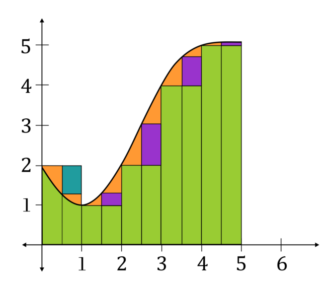
[Left R.S. rectangles have bright red error spaces. Right R.S. rectangles have purple error spaces]
This naturally leads to the question: how can we improve these approximations and minimize error? We can do this by decreasing the width of each rectangle and adding more rectangles in.
Let’s take a look at the same curve’s left rectangles when we decrease their width from one unit to one-half of a unit.
Of course, there are still some error gaps present where either too much or too little area is accounted for. But if we compare this to the previous estimation, we can see that this shaded area has been eliminated, and that these shaded areas have been added in:
So we see that because we increased the number of rectangles, we now have a better approximation of the true value beneath the curve.
Let’s try a formal example now. Consider the function \(f(x)=-x^{3}+25x\). Approximate the area beneath the curve from \(x=0\) to \(x=5\) by finding the left and right Riemann sums, each with five rectangles of width one. Then, find the left and right Riemann sums with ten rectangles of width one-half. Compare each approximation to the true area value, 156.25 square units.
There’s obviously a lot here, so we are going to take this one bit at a time. The function we are working with is \(f(x)=-x^{3}+25x\), and we are looking at the portion of the curve from \(x=0\) to \(x=5\). Our first task is finding the left Riemann sum with five rectangles of width one. This means the left corners of each rectangle will lie on \(x=0\), \(x=1\), \(x=2\), \(x=3\), and \(x=4\) respectively.
Even though we don’t have a picture of the graph in front of us for this problem, we can calculate the heights of those rectangles by plugging those \(x\)-values into the function.
The first rectangle, whose left corner lies on \(x=0\), will have height of:
\(f(0)=-(0)^{3}+25(0)=0\)
The second rectangle’s left corner lies on \(x=1\), so its height will be:
\(f(1)=-(1)^{3}+25(1)=-1+25=24\)
The third rectangle’s left corner lies on \(x=2\), so its height is:
\(f(2)=-(2)^{3}+25(2)=-8+50=42\)
The fourth rectangle’s left corner is at \(x=3\), so its height is:
\(f(3)=-(3)^{3}+25(3)=-27+75=48\)
The fifth and final rectangle has its left corner at \(x=4\), so its height will be:
\(f(4)=-(4)^{3}+25(4)=-64+100=36\)
Each of these rectangles has a width of 1, so their areas, width times height, are each just going to be equal to their height. These areas are again 0, 24, 42, 48, and 36, which all add up to 150 square units.
Let’s now compute the right Riemann sum. For each of the five rectangles, we will need to compute the heights at their right corners.
The first rectangle’s right corner lies on \(x=1\). We’ve already calculated the height at \(x=1\) to be 24, so the first rectangle for the right Riemann sum is then 24 units tall.
The second rectangle’s right corner lies on \(x=2\), and again, we already know the height there. Since \(f(2)=42\), the second rectangle is 42 units tall.
The third rectangle ends at \(x=3\), and will have a height of 48.
The fourth rectangle ends at \(x=4\), and will have a height of 36.
The fifth and final rectangle ends at \(x=5\). We will need to plug this into the function to find the height.
\(f(5)=-(5)^{3}+25(5)=-125+125=0\)
So the last rectangle has a height of 0.
Again, the widths of these rectangles are all 1, so in this case, their areas are simply equal to their heights. Adding all of these together, we see that the right Riemann sum with five rectangles is \(24+42+48+36+0=150\text{ units}^{2}\). Coincidentally, this is the same as the left Riemann sum we got moments ago. For this example, they happened to be the same value; however, this is not always, and often isn’t the case with left and right Riemann sums.
Remember, in the problem statement we were asked to find the Riemann sums using five, and then ten rectangles. Let’s proceed and find the left Riemann sum with ten rectangles now.
Since we are observing the same domain, from \(x=0\) to \(x=5\), increasing the number of rectangles means that we must decrease their width. Now, each rectangle will have a width of one-half. Let’s go ahead and compute the height of the function at intervals of one-half now, so we can calculate the areas and sum more quickly in the next steps:
| \(x\) | \(f(x)\) |
| \(0\) | \(0\) |
| \(0.5\) | \(12.375\) |
| \(1\) | \(24\) |
| \(1.5\) | \(34.125\) |
| \(2\) | \(42\) |
| \(2.5\) | \(46.875\) |
| \(3\) | \(48\) |
| \(3.5\) | \(44.625\) |
| \(4\) | \(36\) |
| \(4.5\) | \(21.375\) |
| \(5\) | \(0\) |
Now, the left rectangles will have left corners at each of these points from 0 to 4.5, so we will be considering each of those heights. In the previous Riemann sums, each rectangle had a width of one, which made calculating the areas very simple. Now, since our rectangles have a width of one-half, each rectangle’s area will be equal to one-half times its height.
So the first rectangle will have an area of \(0.5 \times 0=0\).
The second will have height \(0.5\times 12.375=6.1875\), and so on.
Here are all of the left rectangles’ areas now:
| Rec.1 | Rec.2 | Rec.3 | Rec.4 | Rec.5 | Rec.6 | Rec.7 | Rec.8 | Rec.9 | Rec.10 |
|---|---|---|---|---|---|---|---|---|---|
| 0 | 6.1875 | 12 | 17.0625 | 21 | 23.4375 | 24 | 22.3125 | 18 | 10.6875 |
Adding these all together, we get that the left Riemann sum with ten rectangles is 154.6875 square units.
Now, we are also interested in the right Riemann sum with ten rectangles. From the heights we found, we can again find each of these areas by multiplying the heights by one-half. Here are the areas of each right rectangle, whose right corners are at one-half intervals from \(x=0.5\) to \(x=5\).
| Rec.1 | Rec.2 | Rec.3 | Rec.4 | Rec.5 | Rec.6 | Rec.7 | Rec.8 | Rec.9 | Rec.10 |
|---|---|---|---|---|---|---|---|---|---|
| 6.1875 | 12 | 17.0625 | 21 | 23.4375 | 24 | 22.3125 | 18 | 10.6875 | 0 |
These areas all add up to 154.6875 square units. Even though this value is again the same as what we got for the left Riemann sum, this will not always be the case. This function arcs in such a way that the left and right sums happen to come out equal.
The last part of the problem is for us to compare each approximation to the true area. Using five rectangles, we approximated the area to be 150 square units. With ten rectangles, the approximation was refined to 154.6875 square units. The true area is equal to 156.25 square units. We can clearly see that increasing the number of rectangles in the Riemann sum helped make the approximation more precise!
| Approx with 5 Rec’s | Approx with 10 Rec’s | True Area |
|---|---|---|
| 150 square units | 154.6875 square units | 156.25 square units |
When it comes to Riemann sums, it is important to remember that when calculating the areas of each rectangle, you must multiply its height by its width, which will sometimes be one unit, and other times not. Also keep in mind that these are approximations of the true area beneath a curve. There will still be some margin of error, but this error can be minimized by using more rectangles.
I hope that this video was helpful. Thanks for watching, and happy studying!