Direct Variation

In this video, we are going to discuss a category of functions called direct variation functions, how to write and solve equations involving direct variation, and how to identify examples of direct variation from data given in tables.
By now you’ve seen plenty of examples of functions. Some form flat lines, while others form slanted or even curvy lines. Some pass through the origin, while others do not. The topic of this video is direct variation functions, which are graphically represented as straight lines that pass through the origin.
Algebraically, direct variation functions can be written in the form \(y=kx\), where \(k\) determines the slope of the line. \(k\) can be any number, whether positive or negative, whole or otherwise.
Let’s look at an example of direct variation.
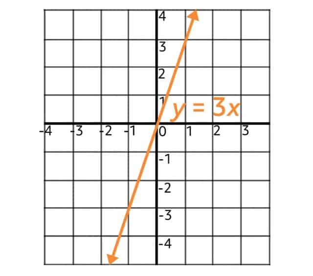
This function satisfies the conditions of direct variation because we can easily see that it is written in the form \(y=kx\). In this case, \(k=3\).
Since this function is an example of direct variation and follows the form \(y=kx\), where \(x\) is raised only to the first power, we are guaranteed that the function is a straight line. Additionally, whenever \(x=0\), \(y=k\times 0=0\), so the line also passes through the origin. Sure enough, this can be seen in the graph of \(y=3x\).
Direct variation functions like these can be helpful in solving real-life problems, as we’ll see in the next example.
Air Force One can fly at the astonishing speed of 600 mph. If the number of air miles traveled by the president is represented by \(y\), and varies directly to the number of hours flown, represented by \(x\), how far would Air Force One travel after 4 hours?
To answer this question, we need to realize that the phrase “varies directly” is used in the problem statement. This means we will use the direct variation formula, \(y=kx\). We are told that \(y\) is the number of miles traveled, and that \(x\) is the number of hours flown. We are also told that the plane travels at about 600 mph. This is our \(k\).
Putting this \(k\) into the direct variation formula, we have \(y=600x\).
miles hours
The amount of time we are concerned with is four hours, so let’s plug in \(x=4\).
Simplifying, we see that \(y=2,400\) miles. That is, after four hours, Air Force One could have traveled an astounding 2,400 miles! That’s the distance from New York to California!
When it comes to direct variation problems, you may sometimes receive information in other forms. Let’s now discuss another type of direct variation problem, where you are given a table of information. To make it clear what kind of information such tables can hold, let’s jump into an example.
Vivian lives on a small hen farm, and each morning she collects eggs to sell at the market. On Monday she gathered and sold 2 dozen eggs for $4.00. On Tuesday she gathered and sold 3 dozen eggs for $6.00. Finally, on Wednesday she gathered and sold 2 dozen eggs for $4.00. We can arrange this information in a table, where one column shows the dozens of eggs sold, and the other shows the amount received.
| Dozens of eggs | Amount received |
| 2 | $4.00 |
| 3 | $6.00 |
| 2 | $4.00 |
Or, if we wanted to present this information in a more clearly mathematical way, we could write the table with the first column called \(x\) and the second called \(y\).
| x | y |
| 2 | 4 |
| 3 | 6 |
| 2 | 4 |
Now that we have arranged the information in this way, it’s time to ask: is this an example of direct variation?
Before we can answer that question though, we need an extra tool. So far, we have been using the form \(y=kx\) to determine whether or not a function is an example of direct variation. But since we don’t have \(y\) written as a function this time, we need to do a slick trick to change \(y=kx\) into something we can use. Notice that from the equation \(y=kx\), we can divide both sides by \(x\) to get \(k\) by itself.
\(\frac{y}{x}=k\)
Now we have that \(\frac{y}{x}\) is equal to \(k\). This is equivalent to the expression \(y=kx\), but we can use it to help us in problems involving tables.
The key to the problem now is solving for \(k\) from each of the three days that Vivian gathered and sold eggs, and then checking whether the values for \(k\) are all the same across all days. If all values of \(k\) are the same, then this is an example of direct variation.
Since Vivian sold 2 dozen eggs for $4.00 on Monday, the \(k\) for Monday is equal to \(\frac{y}{x}=\frac{4}{2}=2\). For Tuesday, she sold 3 dozen eggs for $6.00, so the \(k\) for Tuesday is \(\frac{y}{x}=\frac{6}{3}=2\). Finally, on Wednesday she sold 2 dozen eggs for $4.00, so the \(k\) for Wednesday is \(\frac{y}{x}=\frac{4}{2}=2\).
\(2=2=2\)
\(k=k=k\)
The \(k\) for each day is equal to 2, and since they are all the same, this is indeed an example of direct variation. In fact, now that we know that \(k=2\), we also know that we can write a function describing egg prices per dozen in the form \(y=kx\) as \(y=2x\).
Direct variation has many different applications. Let’s run through one more example to cover the last type of problem you’ll encounter.
Paul has a drippy kitchen faucet, so he leaves a cup underneath it and waters his plants each time it fills up so that no water is wasted. The cup fills once every two hours. Based on this information, write a direct variation equation, and then use it to determine how many times the cup fills after 7 hours.
We need to apply the formula \(y=kx\) to this scenario. Here’s what we have to work with: number of hours passed, times the cup fills up, and the rate at which the cup fills.
Remember in the Air Force One example, we said the speed of the plane was \(k\). In other words, the rate of the plane’s travel was \(k\). When writing direct variation equations, we will always assign \(k\) to be the rate we are given in the problem.
That means that for this problem, \(k\) will represent the rate at which the cup fills up, once every two hours. We write this as
because the cup is halfway full after one hour. Now, we must determine what \(x\) represents and what \(y\) represents. To do this, let’s consider the units of \(k\). \(k\) can be described with the units “cups per hour” because the cup fills one time after two hours.
Now, remember from the previous example that \(k\) is also equal to \(\frac{y}{x}\) in direct variation problems. This tells us that the numerator of \(k\) will have the same units as \(y\) and that the denominator of \(k\) will have the same units as \(x\).
Our direct variation equation is then \(y=12x\), where \(y\) is the number of cups, and \(x\) is the number of hours passed.
Now, we are interested in finding out how many times the cup will fill up after 7 hours pass, so we set hours (\(x\)) equal to 7.
Solving for \(y\), the number of cups, we have
And we are done!
In this video, we’ve learned the two formulas to remember for direct variation are \(y=kx\) and \(k=\frac{y}{x}\). We have also encountered multiple word problems and learned some important phrases to look for, including “varies directly” and “rate” (or the word “per”). For problems involving writing direct variation equations, set \(k\) to be the rate, then notice which units should correspond with \(x\) and with \(y\). With a little practice, you’ll have direct variation mastered in no time.
Thanks for watching, and happy studying!