

Hey everyone! Today we’re going to take a look at standard deviation when applied to a population.
Analyzing Data
Let’s start by looking at what standard deviation can tell us about a set of data.
Let’s say we have a classroom of 100 middle school students, and we measure the height of each student. We now have our data set.
We could find the mean, or simple average, of the data by adding all of the numbers together and dividing by how many students we measured, which in this case is 100. Let’s say the mean height of this group of students is 58 inches tall.
This number alone is quite limited. Without access to the original data, we don’t know if every single student was that height, which would give us that average, or if half of them are 53 inches tall and the other half is 63 inches tall, which also gives us that average.
Normal Distribution
In reality, our intuition would expect there to be a mix of students with most of the students around the average height and fewer students who are a bit shorter or taller and even fewer who are a lot shorter and taller than the average. And our intuition is right. This is what we call a normal distribution, and it looks like this:
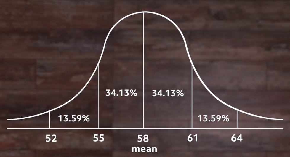
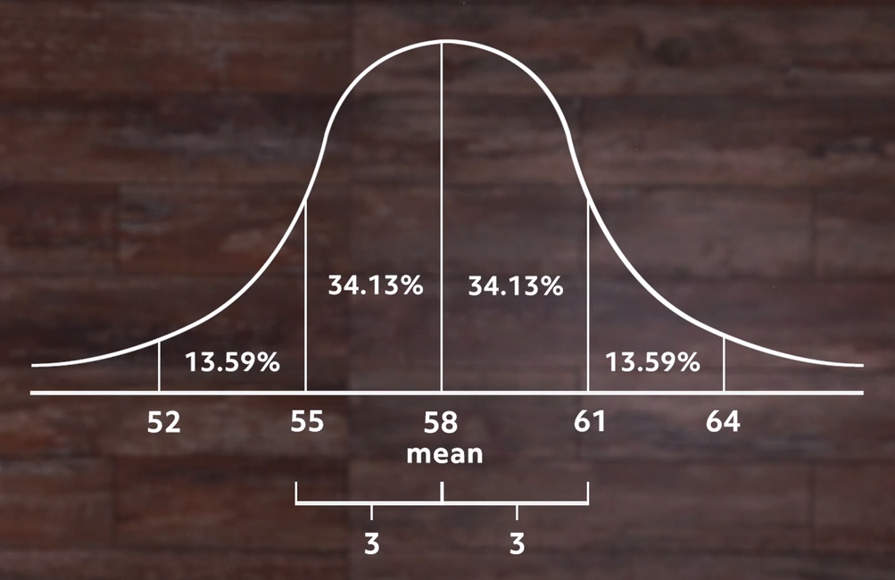
If we start in the center and move to the right until we reach the next vertical line, we’ve moved one standard deviation above the mean, which is the middle. In this example, the standard deviation is 3 inches.
We can see in the area under the graph that this accounts for just over 34% of all the students. If we go back to the middle and move left until we reach a vertical line, we’ve moved one standard deviation below the mean, which accounts for another 34% or so of the students. So we can say that over 68% of the students are within 3 inches (our standard deviation) of the mean height for all the students.
This is always true for a normal distribution. The only thing that changes is the value of the standard deviation itself.
For instance, if we had calculated the standard deviation and it came out to 2 inches instead of 3, then the same percentage of students would be within one standard deviation of the mean, but when we look at the normal distribution it’s taller and we see that our 34% fits within 2 inches of the center rather than 3 like in our previous distribution:
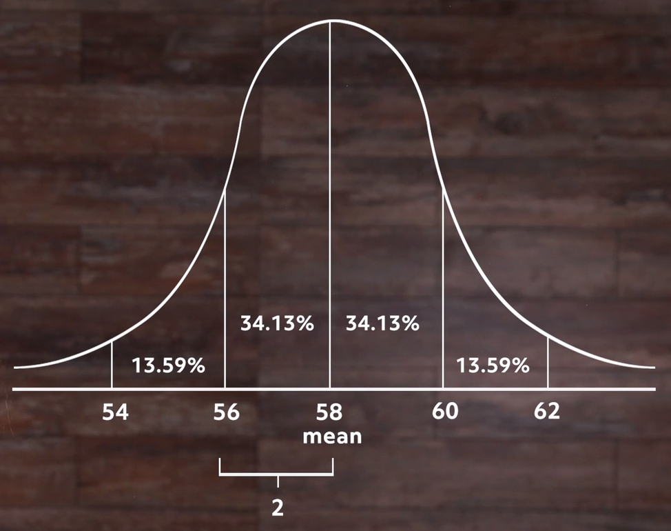
That shows us what standard deviation is all about. In this case, it’s the number of inches of height away from the average that will make up 34% of the population. In the first case it was three inches to account for that percentage of people. In our second example, it only took two inches to account for that percentage.
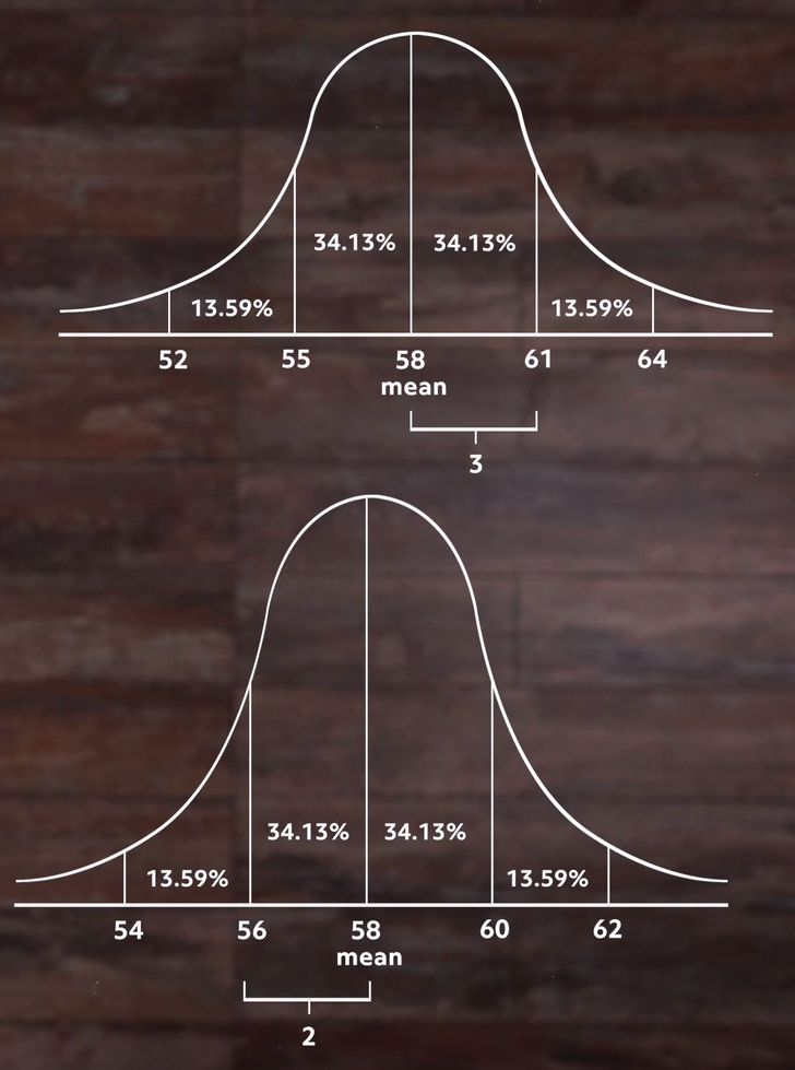
So when we calculate standard deviation from a sample set, that’s what we’re finding. And the number tells us something about all of the data. In our revised distribution we know that most of the students are within two inches, or one standard deviation, of the mean of 58 inches. In our first set, it took a standard deviation of 3 inches to get that many. So you could say it’s a measure of how spread out our data is.
How to Calculate Standard Deviation
So at this point you might be asking: How do we calculate the standard deviation, anyway?
Well, the easiest way is on a spreadsheet, where standard deviation (STDDEV) is a common function that can be used on a range of cells. But we can calculate it manually. Let’s keep our data set small to make our lives a little bit easier. Say we have 10 students and we measure their heights and get values of 52, 55, 56, 56, 57, 58, 59, 61, 62, and 64.
- Step one is to find the mean.
- Step two is to take the difference between each number and the mean and then square it.
\((55 – 58)^2=9\)
\((56 – 58)^2=4\)
\((56 – 58)^2=4\)
\((57 – 58)^2=1\)
\((58 – 58)^2=0\)
\((59 – 58)^2=1\)
\((61 – 58)^2=9\)
\((62-58)^2=16\)
\((64-58)^2=36\)
- Step three is take the average of those squared differences. This is called the variance.
\(0+1+9+16+36=62\)
\(54+62=116\)
\(\frac{116}{10}=11.6\)
So when I add them all up and divide by 10, I get 11.6.
- To find the standard deviation, I simply take the square root of the variance.
The square root of 11.6 is approximately 3.4.
So the standard deviation, in this case, is equal to 3.4 inches. Remember, the standard deviation has units, so that’s inches in this case.
In reality, you probably wouldn’t calculate a standard deviation on such a small population, but this just gives you an idea. The process would still be the same four steps even if there were 1,000 students in your population, though that sure would take a lot longer to calculate manually.
I hope this video was helpful for understanding standard deviation. Thanks for watching. See you next time!
Standard Deviation Practice Questions
For a given data set with a normal distribution, which of the following values for standard deviation will give us the narrowest normal bell curve?
The smallest of these values is 1.5 units, so that is the one that will give us the narrowest bell curve for the normal distribution. Remember, the standard deviation is a measure of how “spread out” the curve will be, with 68% of the population being within one standard deviation from the mean (34% above and 34% below). When those 68% are within just 1.5 units in either direction, the curve is very tall and narrow, compared to larger standard deviations like 25 or 100!
From a given data set, it is determined that the variance is equal to 2,025. What is the standard deviation of the data set?
The relationship between variance and standard deviation is that standard deviation is equal to the square root of the variance.
\(\sqrt{2{,}025}=45\)
In fact, variance is usually written as \(\sigma^2\), because the lowercase Greek letter sigma \((\sigma)\) represents standard deviation.
Over the past four weeks, Deb’s Florist has sold 29, 40, 33, and 36 bouquets each week, respectively. Calculate the standard deviation for this data set. (Hint: start by computing the average, then squaring the difference between each data point and the average. Find the variance by computing the mean of these values, and then take the square root to get the standard deviation.)
First, we compute the average of the four data points.
\(29+40+33+36=138\), and \(\dfrac{138}{4}=34.5\)
The average of the data set is 34.5 bouquets per week. Now, how far is each data point from that average, and what are the squares of those values?
\((29-34.5)^2=(-5.5)^2=30.25\)
\((40-34.5)^2=(5.5)^2=30.25\)
\((33-34.5)^2=(-1.5)^2=2.25\)
\((36-34.5)^2=(1.5)^2=2.25\)
Now that we have these values, we will compute their mean to find the variance.
\(\sigma^2=\)\(\:\dfrac{(30.25+30.25+2.25+2.25)}{4}\)\(\:=\dfrac{65}{4}=16.25\)
Now that we know the variance is 16.25, we just need to take the square root to find the standard deviation.
\(\sigma=\sqrt{16.25}\approx 4.031\)
Carmen is doing research for her taxi company by documenting gas prices in the area over the past 100 days. The average price of gas over the 100-day period was $2.86, and the standard deviation was $0.11. Approximately how many days was the price of gas within $0.11 of the average price?
Remember, we know that approximately 34% of the data points in a set should be between the mean and the value of the mean plus one standard deviation. Similarly, another 34% of the points will be between the mean and the value of the mean minus one standard deviation.
Adding those together, 68% of the data points will be within one standard deviation (plus or minus) from the mean.
Because our data set has one hundred points, we see that 68 points, or 68 days, should be within one standard deviation, or $0.11, of the mean price.
Carlos’s Art Gallery sold four paintings last weekend at auction for the following prices:
- $40,700
- $12,900
- $24,500
- $26,100
Calculate the standard deviation of these prices.
First, we calculate the average of the four prices as follows:
\(40{,}700+12{,}900+24{,}500\)\(\: + \: 26{,}100=104{,}200\), and \(\dfrac{104{,}200}{4}=26{,}050\)
Then, square the difference between each price and the average.
\((40{,}700-26{,}050)^2=214{,}622{,}500\)
\((12{,}900-26{,}050)^2=172{,}922{,}500\)
\((24{,}500-26{,}050)^2=2{,}402{,}500\)
\((26{,}100-26{,}050)^2=2{,}500\)
Now, we take the average of these values to determine the variance.
\(\sigma^2=\)\(\:\frac{(214{,}622{,}500+172{,}922{,}500+2{,}402{,}500+2{,}500)}{4}\)\(\:=97{,}487{,}500\)
Finally, take the square root to find the standard deviation.
\(\sigma=\sqrt{97{,}487{,}500}\approx9{,}873.58\)
The standard deviation of the prices of the four paintings is therefore $9,873.58.